TD-MPC-Glass, Part 23: The Verification Week — What Survived, What Didn't, and Two Config Lines Worth 1.9×
Two weeks ago the plan was to build an ICLR paper on top of the AAAI diagnostic. Before doing that, we re-ran the diagnostic on the official
nicklashansen/tdmpc2rather than our own JAX re-implementation. That verification is this post. It changed the paper — mostly for the better, and not in the direction we expected.
Everything below is read from disk. Where a number is a single run, it says so, because this week taught us exactly how much that matters.
0. Terminology, since we have been sloppy about it
We have been using several words as if they were obvious. They are not.
| Term | What it actually means |
|---|---|
| Arm | One side of an ablation. full = world-model objective on. strip = the same agent with that objective switched off, nothing else changed. |
| Condition / regime | How the training data is collected. This is the thing that turned out to matter most. |
| On-policy | Ordinary RL: the agent acts with its own current policy, so as it learns, the data it sees changes. The two arms end up seeing different data. |
| Matched-data | Both arms act with one shared frozen policy that never learns. Neither arm shapes its own data, so both see the same distribution. The objective is then the only difference. |
| Mis-scoped | A claim that is true but stated more broadly than the evidence supports. Not wrong — over-general. |
| Config lines | Literally lines in a YAML file. No code changes, no new architecture. |
| n=1 / n=3 | Number of random seeds behind a number. This post treats n=1 as a hypothesis, not a result. |
The parameters we keep changing
| Parameter | Lives in | What it does | Default |
|---|---|---|---|
consistency_coef |
TD-MPC2 | Weight on the self-predictive (latent-consistency) loss — the “world model” term we ablate. Setting it to 0 is our strip arm. | 20 |
loss_scales.dyn |
DreamerV3 | The analogous weight on its dynamics loss. 0 is strip. | 1.0 |
iterations |
TD-MPC2 | How many MPPI planning rounds per action. Each round is sequential. | 6 |
horizon |
TD-MPC2 | How many steps ahead the model is trained and rolled out. | 3 |
num_q |
TD-MPC2 | Size of the Q-value ensemble. | 5 |
batch_size |
both | Transitions per gradient update. | 256 |
| update ratio | TD-MPC2 | Gradient updates per environment step. Hardcoded at 1 in online_trainer.py; we patched it to be configurable. |
1 |
One clarification we owe a reader who asked: DreamerV3 is famous for learning from pixels, and it
can. We are deliberately running its dmc_proprio config with env.dmc.image False — i.e. state
observations, to match TD-MPC2’s setup. Every DreamerV3 number in this post is state-based. That
is a choice, not a property of Dreamer.
1. The headline: the claim is real, but it is about the regime
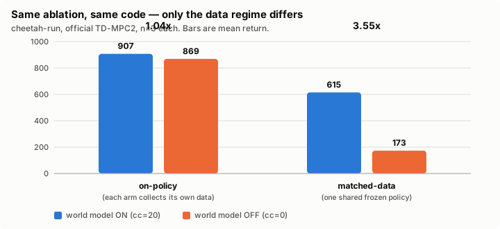
The AAAI draft’s Table 3 reports that removing the self-predictive objective costs ~9.2× on cheetah-run. We re-ran that same ablation on the official implementation under two conditions.
| condition | full | strip | ratio | n |
|---|---|---|---|---|
| on-policy | 907.4 | 869.2 | 1.04× | 3 |
| matched-data | 615.0 | 173.0 | 3.55× | 3 |
| AAAI draft (our old JAX) | 585.6 | 63.8 | 9.2× | 5 |
Per-seed matched-data ratios: 4.60 / 2.94 / 3.36. This is the only major result this week that survived replication, and it survived cleanly.
Reading. Holding the implementation fixed and changing only how data is collected moves the gap from 1.04× to 3.55×. So Table 3 is not a bug — but as written it reads as a fact about cheetah-run, when it is a fact about cheetah-run under frozen-policy data collection. A reviewer reproducing it the ordinary way gets 1.04× and rejects the paper.
Mechanism, which the original did not have. On-policy, the agent explores toward states its reward and value heads already model well, so those heads alone keep the latent dynamics useful. Freeze the behaviour policy and that feedback loop is cut — the self-predictive term becomes the only thing shaping the representation toward states the agent must evaluate.
What we do not claim. The magnitude. Ours is 3.55× against the draft’s 9.2×, and the two setups differ in implementation, coefficient scale (20 vs 2.0), behaviour-policy competence and exploration noise. The defensible phrasing is “several-fold larger under matched data,” not “~9×.”
Two near-misses on this result
Both would have inverted the conclusion:
- The first version of the control was degenerate. Exploration noise decayed linearly to zero, so by 400k the behaviour data was too narrow and both arms starved — full reached 154.5 against ~900 on-policy. It produced 1.57×, which reads as “matched data barely matters.” Fixed with a noise floor of 0.3 plus 10% random-action mixing. This is the same failure mode the original E3c design hit, and it fooled us the same way.
- Our validation test was too strict. We first demanded that both arms collect bitwise identical trajectories. They do not — noise draws differ per process. The control is distribution-matched, not trajectory-matched: collected returns were 745 ± 187 and 709 ± 175 around the frozen policy’s own 723.5 competence. That is the property the control actually needs.
2. Prunability cannot be predicted from importance
This is the result we think is most useful, and it emerged from a hypothesis being falsified.
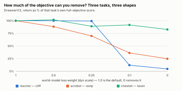
Earlier data hinted that prunability was anti-correlated with importance: reacher, with a huge full-vs-strip gap, tolerated a 4× weight cut for free, while cheetah, with a small gap, did not. So we predicted acrobot — large gap, well measured at 8.79× over 5 seeds — would also tolerate a large cut, and we wrote down the falsifier: if acrobot collapses at 0.25, the reading is dead.
It collapsed.
| task | full-vs-strip effect | retained at dyn=0.25 |
n |
|---|---|---|---|
| reacher | ~57× (largest) | 99% (free) | 3 |
| acrobot | 8.79× | 70% (costly) | 3 |
| cheetah | ~1.25× (smallest) | 89% | 2 |
Order by effect size: reacher > acrobot > cheetah. Order by prunability: reacher > cheetah > acrobot. Acrobot is second on one axis and last on the other, so the relationship is neither correlated nor anti-correlated.
The shapes differ too, which the figure shows better than the table: reacher is a cliff (flat to 0.25, collapsed by 0.1), acrobot a monotone ramp with no threshold at all, cheetah a shallow basin that never leaves 83–102%. A method that assumes one shape — a single global threshold on the loss weight, say — cannot work across tasks.
Why this matters for the paper. The AAAI negative was “world-model benefit is real but not predictable a priori.” This extends it to the actionable question: knowing how much the world model matters tells you nothing about how much of it you can remove. That turns measure-then-prune from a conservative default into the only available method.
3. The acceleration campaign: what actually made it faster
We spent a chunk of the week on wall-clock, and most of our own hypotheses were wrong.
Where the time really goes
The workload is launch-latency-bound. Not compute-bound, not bandwidth-bound.
At the batch sizes these agents use we consume 0.1–3.6% of the GPU’s peak FLOPs and about 9% of
its bandwidth. The decisive measurement: an update costs 23.8 ms at batch 64 and 25.9 ms at batch
1024 — 16× the data for 9% more time. The GPU finishes the arithmetic almost instantly and spends
its time on per-kernel launch overhead. Each environment step fires hundreds of tiny sequential
calls: MPPI alone is iterations × horizon = 6 × 3 = 18 dependent rounds, each evaluating a 5-member
Q-ensemble.
Consequences, each measured rather than assumed:
| lever | result |
|---|---|
Fix the torch.compile recompile storm (TORCHDYNAMO_CACHE_SIZE_LIMIT=256) |
6–10 → 37–40 steps/s |
MPPI depth iterations 6 → 2–3 |
→ ~50 steps/s, and higher return |
| Update ratio 1 → 2 at 2× batch | → ~49 steps/s, return unchanged |
| Pack multiple runs per GPU | 1.25×, and it regresses at 6 |
num_q 5 → 2 (−35% parameters) |
no speedup at all |
| A faster GPU | multiplies FLOPs we do not use |
| Batched physics (MJX) | dm_control already runs 12,474 steps/s on one core; training consumes ~75/s (0.6%) |
Removing arithmetic is free; removing sequential rounds is what pays.
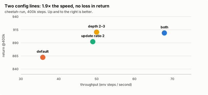
Two config lines, 1.9×
| config | n | return @400k | steps/s | speedup |
|---|---|---|---|---|
| default | 9 | 862.4 (sd 55.8) | ~35.8 | 1.00× |
iterations=2–3 |
4 | 910.6 | ~50 | 1.4× |
| update ratio 2 @ 2× batch | 4 | 892.3 | ~49 | 1.35× |
| both | 3 | 908.9 | 67.9 | 1.90× |
The decomposition is clean. Speedups multiply — 1.4 × 1.35 = 1.89 predicted, 1.90 observed — because the two knobs cut different serial costs. And the return gain comes only from depth: the update-ratio change is neutral on return and pure speed.
On the depth claim specifically, the honest statistic is a rank test, not a mean difference. Pooling every default-config run at a matched window gives n=9, mean 862.4, sd 55.8, range 726–906. All four depth-2/3 runs exceed all nine defaults — under exchangeability that is 1/C(13,4), p = 0.0014. The t-test on means is not significant (t = 1.44), because it is underpowered and the default carries a 726.3 outlier.
Generalisation, with a caveat we like less. On reacher-hard the combined config gives 982.4 and 979.4 against a default of ~982 — equal return at ~1.6–2× speed. So the speedup generalises; the return gain looks cheetah-specific. Both halves belong in the paper.
Depth 1 (729.1) falls inside the default range, so the useful window is 2–3, not “as low as
possible.” And k=4 (one update per four steps at 4× batch) fails on both axes — return collapses to
604 and it is not even faster.
Vectorising the planner: built, gated, and 3.5× — not the 10-30× we estimated
The obvious remaining lever was that official TD-MPC2 runs one environment at a time. Batch N environments through the planner and the sequential MPPI chain is paid once for all of them instead of N times.
We built it as an addition — plan_vec() / act_vec() are new methods; _plan() and act()
are untouched. That shape is deliberate. Our earlier JAX re-implementation of TD-MPC2 diverged from
the official code and cost a week of confusion; keeping the original path intact makes it the
reference rather than a memory.
Correctness gate, run before any speed claim:
| check | result |
|---|---|
N=1 equivalence with _plan under the same RNG |
max|diff| = 0.00e+00 — bit-identical |
| N=16: finite, in [-1,1], non-degenerate spread | PASS |
It surfaced a real bug in the official code on the way: _estimate_value hardcodes
termination = torch.zeros(cfg.num_samples, 1), i.e. it assumes the batch is num_samples.
True for one environment, false for N. Generalised to z.shape[0], which is exactly equivalent in
the original path.
| envs | actions/s | speedup |
|---|---|---|
| 1 | 17.4 | 1.0× |
| 4 | 49.1 | 2.8× |
| 16 | 58.0 | 3.3× |
| 64 | 61.1 | 3.5× |
It saturates at 3.5×, and most of it is there by 4 envs. We predicted 10-30×. That was wrong,
and the reason matters: the MPPI planner is already batched at num_samples=512, so it was
never in the tiny-batch latency-bound regime the update path lives in. At 64 envs its batch is
32,768 latent states — firmly compute-bound. We took “batch is nearly free,” measured on the update,
and over-generalised it to the whole system.
End to end this is worth roughly +20-25% on top of the measured 1.9×, not another order of magnitude.
Why this does not close the gap to Brax PPO
For context we measured MJX on the same GPU: 512 parallel environments give 10M physics steps in 8.9 minutes, reproducing the figure people quote for MuJoCo Playground. Stepping 1 → 4096 environments costs only 4.6× more time while doing 4096× the work.
But that also revealed something we had backwards: at one environment MJX is 119× slower than CPU dm_control (105 steps/s vs 12,474), because GPU launch overhead has nothing to amortise over. The crossover is around 350 environments. So “use MJX” is not a speedup for a single-env agent — it is a speedup for an agent that was already vectorised.
The residual distance to PPO is dominated by the update ratio: TD-MPC2 does one gradient update per environment step, Brax PPO does roughly one per 10³-10⁴. That ratio is TD-MPC2’s sample efficiency, and our own k-sweep bounds how far it can be cut — k=2 free, k=4 costs 604 against 862. PPO needs 10-100× more environment steps to solve the same task. These are two points on a frontier, not a fast method and a slow one.
Correcting our own Part 20
June’s Part 20 concluded that the training bottleneck is gradient updates, not planning, that TD-MPC2 does 64 updates per environment step, and that cheaper planning buys “~zero training speed-up.”
On the official implementation none of that holds. online_trainer.py does one update per env
step, and turning the planner off moves throughput from 43.3 to 66.6 steps/s — planning is ~35%
of training time, not ~0%. The earlier profiling was of our own JAX re-implementation, which
evidently differed in update ratio and in whether data collection goes through the planner.
That is the second time this week our re-implementation and the official code told different stories. It is the reason the whole verification exercise was worth doing.
4. Three findings that died under replication
Worth recording as a group, because the pattern is the lesson.
| claim at n=1 | looked like | after seeds | verdict |
|---|---|---|---|
| Cross-family disagreement on reacher | TD-MPC2 1.01× vs Dreamer 57× | Dreamer’s dyn=0 is past a phase transition; TD-MPC2’s cc=0 is not |
intervention-severity artifact |
| “75% of the objective is free” | cheetah dyn=0.25 ≈ strip |
second seed → mean is intermediate | overstated |
| Walker inversion — the WM hurts | 520.2 vs 611.2 (0.85×) | n=6/arm: 499.3 vs 510.8 | null: 0.98× |
Walker settled the most instructively. As seeds accrued the “effect” decayed monotonically: 0.85× → 0.92× → 0.98×. Nothing about the first measurement was wrong; it was the tail of a distribution we sampled once and reported.
Measured cause. The stripped arm is far noisier than the full arm — in the TD-MPC2 pilot, sd
28.9 against 6.6; on acrobot, van spans 375–419 while strip spans 29–145. Ratios with a
near-zero denominator amplify noise, which is precisely why a dramatic figure like “57×” is
fragile rather than strong.
Consequence for the draft: fix a minimum n per cell, report per-seed values and per-arm spreads rather than ratios alone, and treat any single-seed cell as a hypothesis.
And one open discomfort
Cup-catch (ball-in-cup) is the AAAI draft’s exploration case and its starkest number: 8/14 seeds
versus 0/14. In DreamerV3 we measure van 967.0 (n=2) against strip 944.5 (n=1) — a ratio of
1.02×, essentially nothing. Different framework, so this is not a refutation. But if the world
model is what makes a sparse-reward task solvable at all, one would expect it to show in both.
A second strip seed is running.
5. Proposal: an efficiency paper built on measure-then-prune
The results above suggest a paper we did not set out to write, and we think it is the strongest use of what we now have.
The claim
World-model agents are configured for the hardest case they might meet. Measured per task, most of that configuration is unnecessary — and which part is unnecessary cannot be predicted, only measured. An agent that measures and then prunes runs several times faster at equal return.
Two halves, and each supports the other:
- The diagnostic (the AAAI work, rebuilt on official code): when is the world model actually load-bearing? We now have this across tasks and two model families, plus the finding that prunability is not predictable from importance.
- The lean agent: a configuration whose components — world-model objective, planner depth, update ratio, ensemble size — are individually toggleable, chosen per task by the diagnostic rather than fixed at their defaults.
One structural argument against writing a new algorithm
The instinct is to write a “naive fast world-model algorithm” from scratch. We think that is the wrong move, for a reason this very week demonstrated: a fresh implementation cannot be validated against anything. Our JAX TD-MPC2 diverged from the official code — different update ratio, planner in a different place — and every number built on it had to be re-checked. That cost a week and invalidated a published table.
So the proposal is deliberately not a new codebase. The lean agent is a configuration of the official implementation, plus the vectorised planner we already added and gated:
| component | default | lean setting | evidence |
|---|---|---|---|
planner depth (iterations) |
6 | 2-3 | 1.4×, and higher return (rank test p=0.0014) |
| update ratio | 1 per env step | 1 per 2 at 2× batch | 1.35×, return unchanged |
| world-model objective | on | per-task, from the diagnostic | free on reacher, costly on acrobot |
| planner batching | 1 env | N envs | 3.5×, bit-identical at N=1 |
Q-ensemble (num_q) |
5 | 5 — do not touch | −35% params bought zero speed |
Every row is a measured claim against the official baseline, and every one is falsifiable by rerunning the default. That is the property a from-scratch implementation would lose.
What would make it a paper rather than a config table
- A gate that decides, cheaply. The diagnostic currently costs a full training run per task, which is absurd as a preprocessing step. It needs to be a short probe — a few tens of thousands of steps — that predicts whether the world-model objective pays on this task. We do not know that this is possible, and our own held-out negative is evidence against the easy version. This is the crux and the main risk.
- A frontier, not a point. Report wall-clock against sample efficiency across the sweep, with PPO and the default agent as the endpoints. The honest claim is a better frontier, not “faster than PPO” — PPO wins on wall-clock and loses by 10-100× on samples.
- Breadth. The efficiency numbers are cheetah-heavy. Reacher already shows the speedup generalising but the return gain not. That distinction has to be in the paper, not smoothed over.
What would falsify it
- If the cheap gate cannot beat “always keep the world model” on held-out tasks, the adaptive part collapses and what remains is a config-tuning note, not a method.
- If the lean settings stop being free on harder tasks — humanoid, dog, manipulation — the claim narrows to easy DMC and is not worth a paper.
- If the per-task gains are smaller than seed noise once n is adequate. Given that three separate n=1 findings died this week, this is a live risk and the reason every cell needs seeds first.
Cost
The measurements are mostly done. What is missing is the cheap gate, breadth onto harder tasks, and the frontier plot. On the current two-box fleet that is days, not weeks — which is itself an argument for the paper, since the method is what made the experiments affordable.
6. What this makes the ICLR paper
The AAAI draft was never submitted, so nothing is locked. Our view is that this is now a different and stronger paper, not a patched one:
- World-model benefit is real, task-dependent, and regime-dependent. The regime axis is new and comes with a mechanism.
- Prunability is not predictable from importance — not from effect size, not from task family, not even from curve shape. So measurement is the method, not a fallback.
- A measured efficiency result — 1.9× from two config lines — replacing the draft’s theoretical “~10³× per-action planner cost,” with the honest note that only the speedup generalises.
- A methodology contribution we did not plan: three worked examples of n=1 findings evaporating, with a measured cause.
Two of the three planned world-model families are now covered — TD-MPC2 (value-equivalent) and DreamerV3 (generative). JEPA is the acknowledged gap. DINO-WM-style models build on pre-trained visual features, so that arm is a different observation pipeline rather than another config flag; the realistic near-term version is a state-based JEPA ablation reusing our existing JAX agent.
7. What is running now
- Breadth: four new DMC tasks (finger-spin, hopper-hop, pendulum-swingup, cartpole-swingup-sparse) across both frameworks, taking the prunability claim from 3 tasks to 7. The TD-MPC2 breadth runs deliberately use the default config, not our 1.9× one, so the effect sizes stay comparable to published numbers.
- Replication on every cell that currently carries a claim.
- Prerequisite for a matched-data control on a second task — the experiment that decides whether regime-dependence is general or a cheetah fact. That is the highest-value item left.
Not started: the JEPA arm, and the three-channel separation from the original diagnostic.
Numbers in this post come from 9 default-config runs, 3 matched-data pairs, 4 depth configurations, 3 update-ratio configurations and dose-response sweeps on 3 tasks, all on official implementations. Where n=1, it is labelled n=1.