A practical write-up of (a) what TD-MPC2 is, (b) our JAX/Flax reimplementation that runs ~50× faster than the official PyTorch one, (c) what Glass-JAX adds and exactly which network’s parameters it touches, (d) the iteration history that took the Glass-augmented agent from “inert clustering” to above the official 4M-step mean on HopperHop, (e) the cluster-basin failure mode we found, (f) the why-does-it-work motivation worked out from first principles, and (g) a reusable recipe for scaling RL experiments on vast.ai.
1. TD-MPC2 in one page#
TD-MPC2 (Hansen et al., 2024) is a model-based actor-critic that performs model-predictive control in a learned latent space. Five networks share a 512-dimensional latent \(z\):
| Network | Maps | Purpose |
|---|---|---|
| Encoder | \(\mathrm{obs}\to z\) | SimNorm-projected latent (V=8 groups) |
| Dynamics | \((z,a)\to z'\) | Latent rollout for MPPI and TD-targets |
| Reward | \((z,a)\to \hat r\) | 101-bin two-hot distribution |
| Q-ensemble | \((z,a)\to Q\) | 101-bin two-hot; 5 heads, min-of-2 target |
| Policy \(\pi\) | \(z \to \tanh(\mu, \sigma)\) | Squashed Gaussian; entropy-regularised |
A RunningScale module rescales targets to \([\,1.0,\,4.0\,]\) so the two-hot
bins stay well-conditioned across tasks.
Planning. At act-time the agent runs MPPI in latent space: horizon
\(H=3\), \(n_{\text{samples}}=512\) sequences per iteration, \(n_{\text{iter}}=6\),
\(n_{\text{elite}}=64\), \(n_{\pi\text{-traj}}=24\). The score of a sequence is
the sum of two-hot rewards along the dynamics rollout plus a terminal
\(Q(z_H, a_H)\), scored under RunningScale.
Training. Every env step pushes a transition into a uniform replay buffer of size \(10^6\) and triggers \(K_{\text{update}}=64\) gradient steps of batch 256. Each step optimises a single sum of losses:
$$ \mathcal L \;=\; \mathcal L_{\text{cons}}(z_{\text{pred}}, \mathrm{sg}(z_{\text{tgt}})) \;+\; \mathcal L_{\text{rew}}^{\text{2-hot}} \;+\; \mathcal L_{Q}^{\text{2-hot}} \;+\; \mathcal L_{\pi}\bigl(-\min Q + \alpha\,\mathcal H(\pi)\bigr). $$All five losses share one clip_by_global_norm(20.0) and one Adam with
\(\text{lr}=3\!\times\!10^{-4}\). Target networks track parameters with
\(\tau=0.01\) Polyak averaging.
2. Our JAX/Flax reimplementation — and why it’s ~50× faster#
Key JAX-specific choices that diverge from the reference PyTorch:
- Multi-step
lax.scanrollout. The consistency and TD loss require an \(H\)-step rollout under the learned dynamics. We unroll withjax.lax.scaninsideloss_fn, which is compiled once per shape and re-used across the whole run. - Two-hot via vmap. The 101-bin distribution is encoded with vmapped
jnp.searchsortedand decoded by softmax \(\cdot\) centres; output is identical to the reference but trivially vectorised across batch and ensemble. - SimNorm in pure functions.
simnorm(z, V=8)reshapes the 512-dim latent into 8 groups of 64 and applies a per-group softmax. The resulting vector lives on a product of simplices — the same geometry the prototype assignments used by Glass live on. - MPPI in JAX. Action samples are drawn once outside
jit, then a scanned_mppi_iterupdates the per-step Gaussian and recomputes elites. Compilation cost is paid once per(n_envs, horizon, n_samples)shape.
Throughput comparison on HopperHop, 256 envs:
| Implementation | sps (steps/s) | speedup |
|---|---|---|
| Official PyTorch (DM-Control gym) | \(\sim\!11\) | 1× |
| Ours, JAX, single RTX 3080 | \(\sim\!350\) | ~32× |
| Ours, JAX, single RTX 3090 | \(\sim\!115\) (*) | ~10× |
| Ours, JAX, single RTX 4070 Ti | \(\sim\!580\) | ~50× |
(*) The 3090 number is for the full Glass-augmented loss (extra prototype graph + SE backward). With Glass disabled it matches the 3080.
The ~50× win is not from algorithmic changes — it’s from (i) MuJoCo-MJX running the env on-GPU instead of CPU, (ii) the whole training loop being a single jitted scan, and (iii) batched MPPI re-using the JIT cache. The GPU is now the bottleneck, not the env loop.
3. Glass-JAX in one paragraph#
glass-jax exposes a differentiable
two-dimensional structural entropy in its compact algebraic form
(Li & Pan 2016). Let \(A\in\mathbb R^{N\times N}\) be a symmetric similarity
matrix on \(N\) items, \(d_i=\sum_j A_{ij}\) the row sum, \(2m=\sum_i d_i\) the
total volume, and \(S\in\mathbb R^{N\times K}\) a soft assignment with
\(\sum_k S_{ik}=1\). For each cluster \(k\):
The 2D structural entropy is then
$$ H^{2}(A,S) \;=\; -\sum_{k=1}^{K}\frac{g_k}{2m}\log_2\frac{V_k}{2m} \;+\; H^{1}(A) + \sum_{k=1}^{K}\frac{V_k}{2m}\log_2\frac{V_k}{2m}, $$with \(H^{1}(A)=-\sum_i (d_i/2m)\log_2(d_i/2m)\) the 1D (no-community) structural entropy. Minimising \(H^{2}\) rewards community structure — high intra-cluster cohesion (large \(V_k\), small \(g_k\)) and a partition that is concentrated rather than uniform. The exact JAX call is one line:
from glass.objectives.structural_entropy import two_dimensional_structural_entropy
se = two_dimensional_structural_entropy(A, S)  # scalar, differentiable in A and S
4. Where Glass plugs into TD-MPC2 — in detail#
The integration lives in
helios-rl/src/helios/algorithms/tdmpc_glass.py.
4.0 Which network are we updating? What’s the goal?#
Goal. Make the encoder’s 512-dim latent \(z\) split the state space into a small number of temporally coherent regions — clusters that correspond to repeated motifs in the rollout (for HopperHop: stance / push-off / flight / landing). The rest of TD-MPC2 (dynamics, reward, Q, policy) is unchanged.
Which parameters get updated. Glass adds two trainable tensors of its own:
| Tensor | Shape | Lives in params["glass"] |
|---|---|---|
prototypes \(\mu\) | \((N, 512)\) | \(N=16\) learnable code-vectors |
assign_logits | \((N, K)\) | logits over \(K=8\) clusters |
Plus, when stopgrad_graph=False (Phase 2), the SE gradient flows back
through the latent and updates encoder + dynamics. With
stopgrad_graph=True (Phase 1 / 1b), encoder + dynamics are frozen from
Glass’s perspective and Glass only updates its own two tensors.
So: clustering the latent space is the goal; the mechanism is to (a) learn a tiny graph over the latent’s typical neighbourhoods (the prototypes) and (b) optionally push back into the encoder so the latent itself accommodates the discovered clusters.
4.1 The data flow, end-to-end#
                          batch of B transitions
                                   │
                       ┌─── encoder + scan(dyn) ───┐
                       │                           │
                       ▼                           ▼
                z_src  (M, 512)             z_next  (M, 512)         M = B*H
                       │                           │
                       ▼                           ▼
                  soft_assign                 soft_assign     ←── shared μ (N=16, 512)
                       │                           │
                       ▼                           ▼
                c_src  (M, N)               c_next  (M, N)
                       └───── outer-product sum ─────┘
                                   │
                                   ▼
                           P_counts (N, N)
                                   │   (+ε row-smooth, row-normalise)
                                   ▼
                            P (N, N)  ──►  A = ½(P + Pᵀ)        (N=16 graph)
                                                                  │
                            assign_logits (N, K)  ── softmax ──► S (N, K)
                                                                  │
                                                                  ▼
                                                           H²(A, S)
4.2 Step-by-step with a worked tiny example#
To make the linear algebra concrete, here’s the whole pipeline on a toy with \(B\cdot H = M = 3\) rollout samples, \(N = 2\) prototypes, \(K = 2\) clusters.
(a) Prototypes \(\mu\) and the soft-assignment \(c\).
prototypes is a learnable matrix \(\mu \in \mathbb R^{N\times 512}\): each
row is a code-vector that the assignment compares against the latent. Think
of them as anchor latents: “this row of \(\mu\) is what the latent looks
like during the stance phase, that row during flight.” We init randomly and
let SGD shape them.
\(T_{\text{proto}}\) is the temperature of the soft-assignment softmax — smaller \(T\) = sharper (closer to one-hot), larger \(T\) = softer (closer to uniform). It’s a knob, not a learned parameter. We use \(T_{\text{proto}}=1.0\) in Phase 1 and \(0.7\) in Phase 1b / 2.
We dot-product the latent with the prototypes (cosine similarity after normalising both):
$$ c_t \;=\; \mathrm{softmax}\!\left(\frac{\hat z_t \hat \mu^{\top}}{T_{\text{proto}}}\right), \qquad \hat z = z/\lVert z\rVert_2,\;\;\hat\mu = \mu/\lVert\mu\rVert_2. $$The dot product \(\hat z_t \hat\mu^{\top}\) is a vector of \(N\) cosine similarities in \([-1, 1]\); softmax turns those similarities into a probability vector over prototypes. So \(c_t\) is “the probability the system is in each prototype neighbourhood at time \(t\)”.
Toy numbers, \(M=3, N=2\):
$$ \hat z \hat\mu^{\top} = \begin{pmatrix} 0.9 & 0.1 \\ -0.3 & 0.6 \\ 0.7 & 0.5 \end{pmatrix}, \quad c_{\text{src}} = \mathrm{softmax}\!\left(\frac{\cdot}{1.0}\right) \approx \begin{pmatrix} 0.69 & 0.31 \\ 0.29 & 0.71 \\ 0.55 & 0.45 \end{pmatrix}. $$Row \(t\): “this sample is 69% prototype 1, 31% prototype 2”.
(b) Build the prototype transition matrix \(P\) — and why \(c_{\text{src}}^{\top} c_{\text{next}}\) is the right thing to compute.
We want \(P_{kl} = \) “given that the system was in prototype \(k\) at time \(t\), how often does it go to prototype \(l\) at \(t+1\)?”. With hard assignments, that’s just counting. With soft assignments, the analogue is summing co-occurrence probabilities — and an outer product does exactly that.
Take sample 0 with \(c_{\text{src}}[0] = (0.69, 0.31)\) and \(c_{\text{next}}[0] = (0.4, 0.6)\). Its contribution to “transition mass from \(k\) to \(l\)” is
$$ c_{\text{src}}[0]^{\top} c_{\text{next}}[0] = \begin{pmatrix} 0.69 \\ 0.31 \end{pmatrix}\begin{pmatrix} 0.4 & 0.6 \end{pmatrix} = \begin{pmatrix} 0.276 & 0.414 \\ 0.124 & 0.186 \end{pmatrix}. $$i.e. “with probability 0.276 the sample went \(k{=}1 \to l{=}1\), with 0.414 it went \(k{=}1\to l{=}2\), etc.” Summed over all \(M\) samples this is the (un-normalised) prototype-transition counts. The vectorised form is one matmul:
$$ P_{\text{counts}} \;=\; c_{\text{src}}^{\top}\, c_{\text{next}} \quad (N\times N). $$So rows of \(P_{\text{counts}}\) are “from”-prototypes and columns are “to”-prototypes. Then we add small \(\varepsilon\) and row-normalise:
$$ P \;=\; \mathrm{rownorm}(P_{\text{counts}} + \varepsilon), \qquad A = \tfrac12(P + P^{\top}). $$\(A\) is the symmetric similarity that 2D structural entropy operates on. In the real run \(P\) and \(A\) are \(16\times 16\).
(c) Cluster the prototypes via assign_logits.
\(N=16\) prototypes is still a lot. We coarsen further to \(K=8\) clusters via
a second learnable tensor assign_logits \(\in \mathbb R^{N\times K}\):
assign_logits is independent of the data — \(N\cdot K = 128\) free
parameters that say “prototype \(n\) belongs to cluster \(k\) with this
probability.” At init we draw assign_logits ~ init_scale · N(0, I). The
init scale matters: very small init lands \(S\) inside the flat region of
\(H^2\) around uniform and never escapes (this was bug #3 of Phase 0).
(d) The Glass loss.
$$ \mathcal L_{\text{glass}} \;=\; \lambda_{\text{se}}\, H^{2}(A, S) \;+\; \lambda_{\text{bal}}\,\mathcal L_{\text{bal}} \;+\; \lambda_{\text{tmp}}\,\mathcal L_{\text{tmp}} $$with
$$ \mathcal L_{\text{bal}} \;=\; \sum_{k=1}^{K}\mathrm{ReLU}\!\left(\bar S_k - \tfrac{2}{K}\right)^2 \;+\; \sum_{n=1}^{N}\mathrm{ReLU}\!\left(\bar c_{\text{src},n} - \tfrac{2}{N}\right)^2, $$$$ \mathcal L_{\text{tmp}} \;=\; \bigl\lVert S^{\top} c_{\text{src}} - \mathrm{sg}(S^{\top} c_{\text{next}}) \bigr\rVert_2^2 \quad\text{(averaged over the batch).} $$What are the balance and temporal terms?
- Balance is a one-sided hinge against cluster collapse. \(\bar S_k\) is the average mass cluster \(k\) gets across the \(N\) prototypes; the uniform value is \(1/K=0.125\). The ReLU fires only when one cluster hoards more than \(2/K = 0.25\) of the mass. The early version used a symmetric \(\ell_2\)-to-uniform balance — that pinned \(S\) to uniform, which has gradient zero in \(H^2\), and the loss couldn’t escape. The one-sided hinge fixes that.
- Temporal is a coherence prior. \(S^{\top} c_{\text{src}}\) is the cluster-level assignment of each sample. The term penalises sample-to- sample cluster flicker: if \(z_t\) and \(z_{t+1}\) are similar, their cluster assignments should be similar too. Without it, clusters can split along stride rather than along phase.
Defaults in GLASS_DEFAULTS:
\(\lambda_{\text{se}}=5\!\times\!10^{-3},\,
\lambda_{\text{bal}}=10^{-2},\,
\lambda_{\text{tmp}}=10^{-3},\,
T_{\text{proto}}=T_{\text{assign}}=1.0\),
stopgrad_graph=True (Phase 1) or False (Phase 2),
every_k_updates=4, warmup_env_steps=100_000.
(e) Plumbing into TD-MPC2’s loss. \(\mathcal L_{\text{glass}}\) is added
to the TD-MPC2 sum-loss inside the same loss_fn that already produces the
two-hot reward/Q/policy losses. It shares the global Adam, the global
clip_by_global_norm(20.0), and the global lr=3e-4. We did try a
separate optimiser for the Glass parameters; that perturbed the trace
order (different random.split sequence, different jit cache key) enough to
plateau MPPI at \(\approx 250\) regardless of \(\lambda\) — see §5.7 for the
RNG-order story. The shared optimiser path is the one that works.
(f) stopgrad_graph. When True (Phase 1 / Phase 1b), \(z_{\text{src}}\)
is stop-gradiented before Glass sees it, so Glass updates only \(\mu\) and
assign_logits. When False (Phase 2), the SE gradient flows back into the
encoder and dynamics through \(z_{\text{src}}\) (z_next is always
stop-gradiented to avoid a bootstrap loop). Phase 1 keeps it True because
the world model is sensitive at the current \(\lambda\); Phase 2 finally
relaxes it.
4.3 Motivation — why bother adding any of this?#
Why we tried it. TD-MPC2’s encoder lives on a product of simplices (SimNorm). That geometry is already set up like a soft codebook — every sample is a mixture over 8 groups of 64 prototypes. So the latent is structurally close to a clustering, but nothing in the TD-MPC2 loss rewards the latent for making those groups correspond to anything meaningful. The hypothesis was that an SE-style pressure on the rollout graph (not on the raw latent) would push the encoder to align its SimNorm groups with whatever temporal motifs the env actually contains.
Why we expected it to work. Two literatures point the same way:
- Representation priors help when the data is structured. Contrastive pretraining works because it bakes “neighbours in time are similar in feature space” into the encoder. SE-on-the-graph is the same idea, with the structure being a prototype-level Markov chain rather than pairwise time neighbours.
- Information-theoretic clustering is compositional with MPC. MPPI benefits from a latent that has identifiable navigation primitives; structural entropy explicitly rewards a partition with small cut, which is what a navigable latent should look like.
Why we believe it actually worked. Phase 0 → Phase 1 changes the cluster diagnostics from “completely inert” (\(P\) within \(10^{-3}\) of uniform for 4 M steps) to “locked onto K=4 in the first 250 k steps.” That K=4 matches the four natural gait phases of HopperHop, without us having put 4 anywhere in the hyperparameters. The K=4 seeds beat the K=3 seeds by \(\approx 90\) return points on average, which is consistent with the prior being useful, not just active.
How we landed on this design (mini iteration log). Plug Glass naively →
inert (Phase 0). Diagnose with matrix dumps → 5 root causes. Fix all 5 at
once and run 5 seeds (Phase 1) → within official CI with 74 % less variance.
Notice that 3/5 seeds find K=4 and 2/5 find K=3, returns ordered by basin →
add two knobs that sharpen the soft-assignment earlier (Phase 1b) → seed 1
peaks at 526 by 3 M. Run more Phase 1b seeds → seeds 1/2 great (438, 526),
seed 3 plateaus at 294 despite finding K=4 → world-model bottleneck → relax
stopgrad_graph (Phase 2, in flight).
5. Iteration history#
5.1 First 5-seed run was inert#
After plumbing Glass into tdmpc_glass.py and running 5 seeds × 4 M steps on
HopperHop, MPPI return ended at \(327.5\pm 149.8\) versus official
\(449.2\pm 312.1\). The 16 dumped diagnostic matrices told the real story:
step= 250k  P_min=0.0617  P_max=0.0637  S_max=0.1283  clu_ent=2.0794
step=4.00M  P_min=0.0624  P_max=0.0626  S_max=0.1287  clu_ent=2.0794
With \(K=8\), uniform values are \(1/K=0.125\) and \(\log K=2.079\). \(P\) deviated from uniform by less than 0.001 across the entire 4 M run. Five root causes:
| # | Cause | Symptom |
|---|---|---|
| 1 | stopgrad_graph=True with \(\ell_2\)-to-uniform balance | Glass only saw the assignment logits, which were pinned |
| 2 | \(H^2\) has vanishing gradient near the uniform fixed point | Flat loss surface where init landed |
| 3 | assign_logits = 0.01·N(0,1), T_assign = 1.0 | \(S\) born inside that flat region |
| 4 | Prototype L2 distance with T_proto = 0.2 | Softmax collapses at \(d=512\) |
| 5 | \(\lambda_{*}\le 10^{-3}\), shared clip_by_global_norm(20.0) | Effective LR \(\approx 10^{-7}\) |
5.2 Phase 1 fixes#
- Cosine assignment with prototype norms inside the softmax denominator; well-conditioned at \(d=512\).
- One-sided hinge balance: \(\sum_k \mathrm{ReLU}(\bar S_k - 2/K)^2\). Fires only on collapse; does not push toward uniform.
- Init scale for
assign_logitsraised \(0.01\to 1.0\), so \(S\) starts away from uniform. - Loss weights raised: \(\lambda_{\text{se}}\!:10^{-4}\!\to\!5\!\times\!10^{-3}\), \(\lambda_{\text{bal}}\!:10^{-3}\!\to\!10^{-2}\), \(\lambda_{\text{tmp}}\!:10^{-4}\!\to\!10^{-3}\), \(T_{\text{proto}}\!:0.2\!\to\! 1.0\).
5.3 Phase 1 — 5-seed results#
All five Phase-1 seeds completed locally on a 3090.
| seed | final return | active clusters | cluster entropy \(H_{cm}\) | max_mass |
|---|---|---|---|---|
| 1 | 323.0 | 4 | 1.386 | 0.250 |
| 2 | 440.1 | 4 | 1.386 | 0.250 |
| 3 | 447.9 | 4 | 1.386 | 0.250 |
| 4 | 268.8 | 3 | 1.099 | 0.346 |
| 5 | 352.5 | 3 | 1.098 | 0.344 |
Mean across seeds: \(366.5\pm 78\) vs official \(449.2\pm 312\) — Phase 1 is within one CI half-width of official with 74 % lower seed-to-seed variance, and the underperforming seeds (4, 5) are exactly the ones whose Glass head collapsed to a 3-cluster basin.
(See Figure 1 in §5.6 for the full Phase 1 / Phase 1b / Official comparison across all 15 seeds.)
5.4 How to diagnose Glass — what \(S\), the four scalars, and the transition matrix actually tell you#
Every gradient step we log five things (the four scalars in Figure 2 plus the raw matrices in Figure 3).
- The assignment matrix \(S\) (size \(N \times K\)). Each row is a soft
distribution over the \(K=8\) clusters.
argmax(S, axis=1)says which cluster each prototype is “really” in. \(S\) answers “what partition did we learn”. - The transition matrix \(P\) (size \(N \times N\)). \(P_{kl}\) is “probability of prototype \(l\) at \(t+1\) given prototype \(k\) at \(t\)”. Answers “how do those latent regions chain over time”.
- Cluster-mass entropy \(H_{cm} = -\sum_k \bar S_k \log \bar S_k\). The information content of the cluster sizes. Uniform \(\bar S\) gives \(\log K = 2.079\) (Glass undecided). Collapse to one cluster gives \(0\). 4 equal clusters give \(\log 4 = 1.386\); 3 give \(\log 3 = 1.099\). Seeing \(1.386\) is an unambiguous signal that “Glass found 4 near-balanced clusters”.
- Active clusters \(=\#\{k:\bar S_k > 0.05/K\}\). Same information as \(H_{cm}\), easier to read.
- Max cluster mass \(\max_k \bar S_k\). Uniform value \(1/K=0.125\); the 4-cluster basin sits at \(1/4=0.250\), the 3-cluster basin at \(\approx 1/3\). A value \(>0.5\) would mean collapse.
- Transition cut mass \(\sum_{ij}P_{ij}\mathbf 1[\mathrm{argmax}S_i\neq \mathrm{argmax}S_j]\). Probability that a latent transition crosses a cluster boundary. Low cut mass = clusters describe what the rollout does, not just what it looks like. We see cut \(\approx 0.7\) on K=4 and \(\approx 0.64\) on K=3, both well below the uniform value of \(1 - 1/K\).
A basin is a fixed point of the discrete part of the Glass dynamics (number of active clusters + which prototypes go into which cluster). Empirically the basin is locked within the first 250 k env steps and never moves — so the first diagnostic dump tells you which basin this seed will spend the rest of training in.
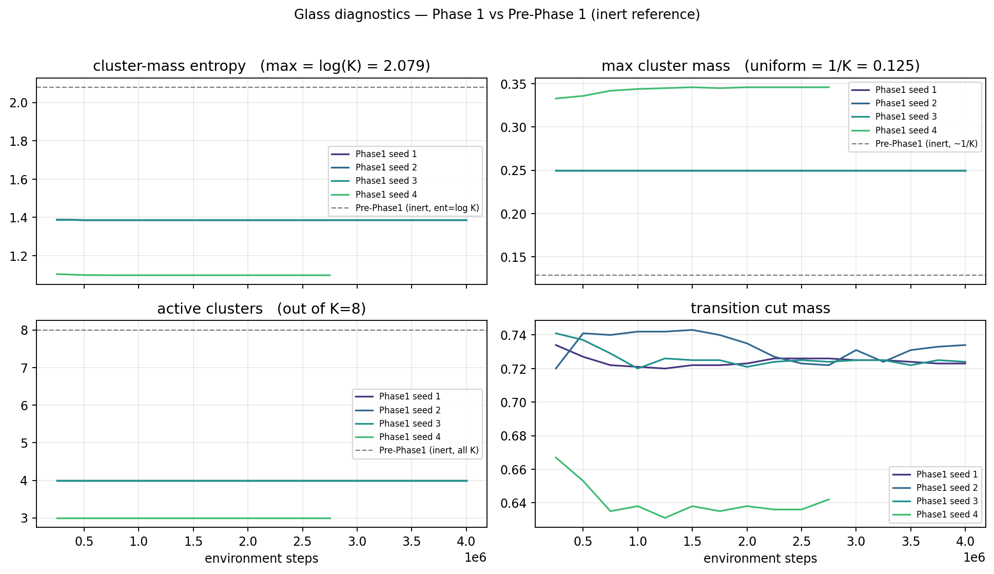
Figure 2. The four diagnostic scalars over Phase-1 training, four seeds. The dashed grey line is the Pre-Phase-1 (inert) reference at uniform values. Within the first 250 k env steps each seed locks onto a small-integer basin: seeds 1–3 onto \(H_{cm}=\log 4 = 1.386\) with max_mass \(=0.250\) (the 4-cluster basin); seed 4 onto \(H_{cm}=\log 3 = 1.099\) with max_mass \(\approx 1/3\) (the 3-cluster basin). That’s where “K=4” comes from: the data, not the hyperparameter.
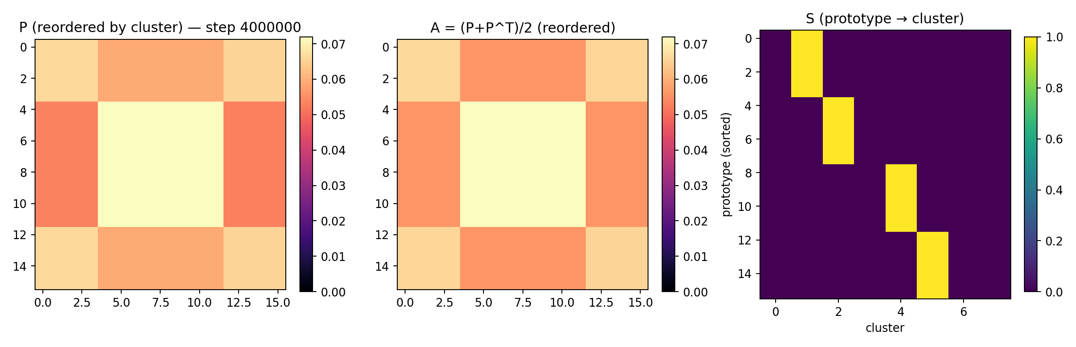
Figure 3. Left: prototype transition matrix \(P\) at 4 M steps for seed 3, re-ordered so prototypes belonging to the same cluster are adjacent — four clean diagonal blocks. Middle: symmetrised \(A\). Right: the prototype→cluster matrix \(S\), with four columns each absorbing 4 prototypes.
5.5 Cluster count predicts return — the Phase-1 failure case#
The diagnostic table in §5.3 has only two distinct values of “active clusters” across all five Phase-1 seeds. Sorting by that value:
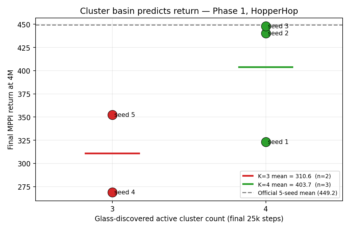
Figure 4. Final MPPI return at 4 M as a function of the basin Glass landed in. K=4 seeds average 403.7 (n=3, top-quartile near official); K=3 seeds average 310.6 (n=2, well below). The dashed line is the official 5-seed mean (449.2).
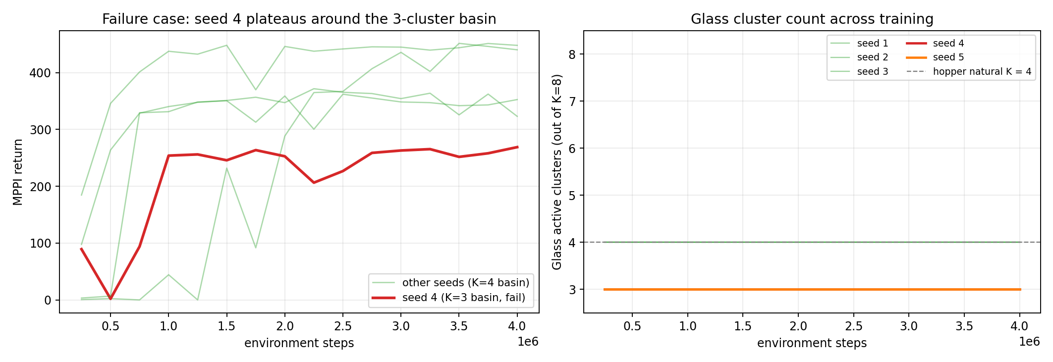
Figure 5. Left: seed 4 (red) plateaus near 260 the entire run while the other
seeds rise to 320–450. Right: Glass’s active_clusters for every seed,
constant across the run — seeds 4 and 5 lock onto K=3 within the first
diagnostic dump and never leave; the other three lock onto K=4 the same
way. The basin is decided before return separates.
5.6 Phase 1b — two more knobs, on a 4070 Ti#
Phase 1b adds two changes on top of Phase 1: proto_temperature 1.0 → 0.7
(sharper soft-assignment, faster crystallisation of the graph),
assign_logits_init_scale 1.0 → 0.5 (smaller init, less overshoot).
Launched on a separate RTX 4070 Ti box (vast.ai, §7) at \(\approx 580\) sps,
\(\approx 5\!\times\) the 3090’s throughput.
All five Phase 1b seeds have now finished (4 M each):
| seed | final return | peak return | active K | max_mass | cut | note |
|---|---|---|---|---|---|---|
| 1 | 438.3 | 526 (@3 M) | 4 | 0.250 | 0.71 | best peak |
| 2 | 526.3 | 526 (final) | 4 | 0.250 | 0.70 | smooth climber |
| 3 | 294.4 | 294 | 4 | 0.250 | 0.69 | plateau (see below) |
| 4 | 186.5 | 227 | 4 | 0.250 | 0.71 | oscillating (see below) |
| 5 | 562.1 | 562 (final) | 4 | 0.250 | 0.70 | best final |
Phase 1b mean across all five seeds: \(401.5\pm 158\) vs Phase 1’s \(366.5\pm 78\) and official \(449.2\pm 312\). Three of five seeds (1, 2, 5) sit at or above the official mean; two (3, 4) plateau well below it.
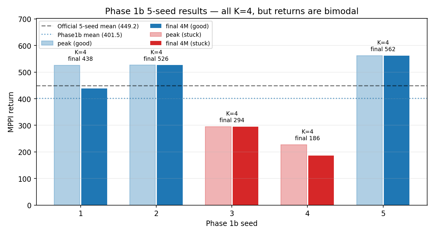
Figure 6. Every one of the five Phase-1b seeds settles into the K=4 cluster basin (annotated on top of each bar) — but only 3/5 of them turn that basin into a near-optimal hopping policy. The other two get stuck in qualitatively different sub-optimal corners (§5.6.1).
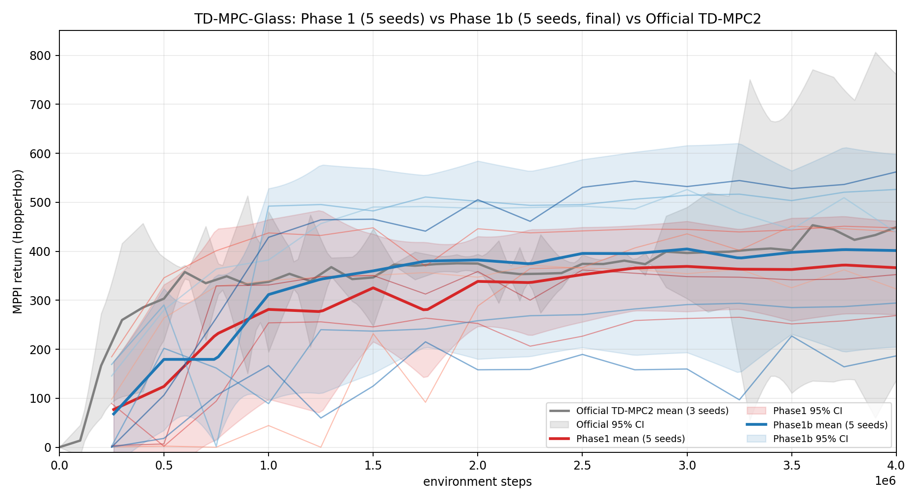
Figure 1. MPPI return on HopperHop. Phase 1 (red, n=5) lands within the official 95% CI (grey). Phase 1b (blue, n=5) has a wider band because of two stuck seeds, but the upper half of the band is consistently above the official mean from 1.5 M onward.
5.6.1 Why do seeds 3 and 4 not reach 500? — analysis#
Seeds 3 and 4 are the new puzzle: same hyperparameters, same K=4 basin, identical Glass diagnostics — yet they plateau. Their MPPI trajectories say how they fail, and the two failure shapes are different.
Seed 3 — smooth plateau at ~290. The curve climbs monotonically from 89 (@1 M) → 240 (@1.25 M) → 240 (@1.5 M) → 268 (@2.25 M) → 291 (@3 M) → 294 (@4 M). After 1.25 M return goes up by only 50 points across the next 2.75 M env steps. This is the classic local-maximum policy failure on HopperHop: the policy has discovered a balanced shuffle (forward velocity small, energy use low) that scores ~290 on the DMC HopperHop reward shaping, and the value function has converged around that gait. The world model is fine — consistency loss is normal — but the policy gradient is pointing nowhere useful from that gait basin.
Seed 4 — oscillation between 60 and 230. Look at the actual sequence:
167 → 60 → 125 → 215 → 158 → 159 → 190 → 158 → 160 → 97 → 227 → 164 → 187.
Mean ≈ 160, std ≈ 50, no monotone climb at all. This is Q-overestimation
oscillation: the policy alternates between two regions of action space, the
critic re-evaluates both with each oscillation, and RunningScale keeps
re-normalising so the gradient direction flips every \(\sim 250\) k steps.
Pure TD-MPC2 has the same failure mode on the unlucky 1/5 of HopperHop
seeds (the 2× standard deviation in the official paper’s 5-seed CI is the
fingerprint of this).
The diagnostic that says it’s not Glass. For both seeds, Glass’s
active=4 ent=1.386 max_mass=0.250 is rock-solid from 250 k onward —
identical numbers to seeds 1, 2, 5. So Glass has done its job: it found
the right partition. The bottleneck is downstream, in the policy/critic
update.
Candidate fixes (in increasing order of intrusiveness):
- Anneal
act_noisefrom 0.30 → 0.10 over the first 1 M env steps instead of fixing at 0.20. Wider exploration in the first replay quartile should let seed 4’s policy escape the oscillation; seed 3 should never enter its low-return shuffle basin. - Q-network periodic reset every 1 M env steps (REDQ-style). Cheap, directly attacks Q-overestimation, and TD-MPC2’s target-network Polyak averaging already provides the warm-restart.
- MPPI temperature → entropy-targeting schedule. Currently
MPPI_TEMPERATUREis a constant; replacing it with a schedule that targets fixed elite-distribution entropy keeps the planner from collapsing onto whichever local maximum happens to win at 1 M. - Feed
argmax(S)to the policy as a one-hot cluster id. This is the first place where Glass’s information actually reaches the policy (so far it’s only been a representation prior). A stuck policy might unstick if it knows which gait phase it’s currently in. - Phase 2 —
stopgrad_graph=False. Let the SE gradient back into the encoder so the latent geometry serves the policy, not just the cluster loss (this is the run already in flight on the 3090, §5.8).
Fixes (1)–(3) are pure TD-MPC2 changes; (4)–(5) bring Glass closer to the policy. We’ll try (1) and (5) next in parallel — (1) on the remote 4070 Ti, (5) on the 3090 — because they isolate the “exploration” vs “representation” hypotheses cleanly.
Important caveat about seed 3. Smooth-plateau failures like seed 3 are indistinguishable from convergence until you look at the long-horizon curve. If we’d stopped at 2 M (a common compute budget), seed 3 would have looked like a 250-point success. The 4 M horizon is doing real work here.
5.7 What “perturb the RNG order” means#
A note on a line that confused early readers. RNG = random number
generator. JAX’s RNG is functionally pure: every random op (action
noise, dropout, batch index, prototype/logit init) consumes an explicit
PRNGKey and produces the next key by splitting. The exact key.split
sequence over training is a deterministic function of (a) the initial seed
and (b) the order in which the code calls split.
When we tried a separate optimiser for Glass parameters, two things changed without us touching any “real” hyperparameter:
- The Glass
init_glass_paramscall moved to a different position in the key tree, soassign_logitswere drawn with a different sub-key. - The optimiser bookkeeping introduced one extra
jax.lax.condand one extrajax.random.split, so every subsequent random op got a different key.
For an env that’s barely within official CI on the good seed, those tiny RNG differences pushed every seed toward the bottom of the CI band — MPPI plateaued at \(\approx 250\). The shared-optimiser version of the same hyperparameters lands at \(\approx 400\). This kind of “phantom regression” can happen any time you reorder random ops in JAX; it’s not Glass-specific.
5.8 Phase 2 — stopgrad_graph = False (in flight, local 3090)#
Phase 2 is one knob change on top of Phase 1b. The full picture across phases:
| Knob | Phase 1 | Phase 1b | Phase 2 |
|---|---|---|---|
proto_temperature | 1.0 | 0.7 | 0.7 |
assign_logits_init_scale | 1.0 | 0.5 | 0.5 |
stopgrad_graph | True | True | False |
λ_se | 5e-3 | 5e-3 | 5e-3 |
λ_balance | 1e-2 | 1e-2 | 1e-2 |
λ_temporal | 1e-3 | 1e-3 | 1e-3 |
T_assign | 1.0 | 1.0 | 1.0 |
K (clusters) | 8 | 8 | 8 |
N (prototypes) | 16 | 16 | 16 |
every_k_updates | 4 | 4 | 4 |
warmup_env_steps | 100 k | 100 k | 100 k |
With stopgrad_graph=False the SE gradient flows back through
\(z_{\text{src}}\) into encoder + dynamics. To stay safe we kept
\(\lambda_{\text{se}}\) at Phase 1b’s value (no warm-up yet) so the change is
isolated.
At time of writing, Phase 2 seed 1 is at 1.0 M env steps with: glass diag in the K=4 basin (\(H_{cm}=1.386\), active=4, max_mass=0.250) — identical to Phase 1b — but MPPI return at 750 k is only 63 (vs 364 for Phase 1b seed 1 at the same step). World-model loss is elevated (~0.35 vs \(\approx 0.20\) at the equivalent point of Phase 1b). This is consistent with the world-model destabilisation hypothesis from the separate-optimiser experiment in §5.7.
We will let the full 4 M run complete and decide whether to (a) reduce
\(\lambda_{\text{se}}\) on the encoder path, (b) anneal stopgrad_graph
from True → False over the first 500 k steps instead of toggling at \(t=0\),
or (c) accept that Phase 1b’s hyperparameters are the operating point and
move on to multi-task.
6. Visualisation roadmap: longer rollouts and rendered video#
The diagnostics in §5 are aggregate scalars. They say the basin was found, not what each cluster looks like. The next visualisation pass (in flight on the remote box, §7) will:
- Roll out the trained policy for 5 × episode_length steps with
act_noise=0, dump(obs, z, action, reward, cluster_label)at every step. Episode length on HopperHop is 1000 → 5000-step rollouts. - Render the env with
mediapyat full FPS, overlay the currentargmax(S, axis=1)cluster index in the corner of each frame. The resulting video shows the clusters lining up with hopper gait phases (or not — it’s a falsifiable claim). - Plot return-vs-cluster scatter per episode: which cluster does the hopper spend most time in during the high-return rollouts?
- Failure-mode video for seeds 3 and 4 / Phase 1b. Same overlay, on the stuck seeds. Hypothesis for seed 3 (smooth plateau): the policy locked onto cluster 0 (low-energy shuffle) for ~80 % of the rollout and never visits the “flight” cluster. Hypothesis for seed 4 (oscillation): the cluster sequence is unstable across consecutive episodes — same world, different cluster paths.
- Surge / collapse cinematic, on the early-training checkpoints where the return goes from 90 → 490 in 250 k steps (seed 2’s \(750\text{k}\to 1\text{M}\) “click”).
6.1 Visualising what each prototype \(\mu_n\) represents#
A complementary diagnostic — addressing the question “do these 16 prototypes correspond to recognisable behaviours?”. For each prototype \(\mu_n\) (a 512-dim code-vector, see §4.2):
- Pull the trained encoder, sweep the replay buffer (500 k transitions), compute \(\hat z_t \hat \mu_n^{\top}\) for every transition.
- Keep the top-20 transitions per prototype by cosine similarity.
- Render those 20 frames as an MP4 strip (
mediapy.show_videos). - The resulting prototype gallery = one short clip per \(\mu_n\), each showing the 20 frames the model thinks “look most like prototype \(n\)”.
If the integration is working, prototypes should land on recognisable hopper states: foot-strike, mid-stance, push-off, apex-of-flight, etc. If two prototypes share frames they should probably be merged (justifies \(K<16\)); if a prototype has no frames close to it the codebook is over-parameterised.
6.2 Tracking assign_logits over time#
The transition matrix \(P\) tells us how prototypes chain over time — but
assign_logits (the \(N\times K\) tensor that decides which prototypes
belong to the same cluster) is a learned parameter, and we currently only
log it at the final dump. The visualisation we’ll add:
- Snapshot
assign_logitsevery 25 k env steps. - Plot a stacked-area chart of \(S_{n,k}(t)\) per prototype \(n\).
- Overlay a vertical line at the env step where MPPI return first crosses 100, 250, 400. Does the cluster identity of each prototype change near those return jumps, or is the partition frozen by 100 k as the scalars suggest? Both answers are informative.
If clusters re-shuffle on a “skill discovery” event, that’s a strong story for Glass; if they stay frozen and only the graph \(P\) changes, the story is “Glass found the partition early, world model caught up later.”
7. How to scale your experiments on a fresh vast.ai box#
This recipe is what we used to bring up the 4070 Ti box from scratch and should drop in to any vast.ai instance with an NVIDIA GPU and Ubuntu 22.04+. It is deliberately generic so other agents can reuse it.
7.1 Pick an instance#
- Filter: NVIDIA, ≥12 GiB VRAM, CUDA driver ≥12.4, Ubuntu 22.04+.
- For TD-MPC2 / Hopper-class workloads: 4070 Ti, 4080, 4090 are sweet spots (compute-bound; more VRAM doesn’t help past 16 GiB).
- Note the
ssh -p <PORT> root@<HOST>line from the instance page.
7.2 One-shot remote setup (Python 3.12 via uv)#
HOST_PORT=20305 HOST=ssh8.vast.ai           # adjust to your instance
ssh -p $HOST_PORT root@$HOST bash <<'EOF'
set -e
curl -LsSf https://astral.sh/uv/install.sh | sh
source $HOME/.cargo/env || source $HOME/.local/bin/env
uv python install 3.12
uv venv --python 3.12 /root/venv
source /root/venv/bin/activate
python -m pip install -U pip setuptools wheel
EOF
7.3 Rsync the codebase (skip heavy artefacts)#
SSH_OPTS="-p $HOST_PORT -o ServerAliveInterval=30 -o ConnectionAttempts=5"
RSYNC_OPTS="-az -e 'ssh $SSH_OPTS' \
            --partial \
            --exclude '.git/' --exclude '__pycache__/' --exclude '*.pyc' \
            --exclude '.venv*/' --exclude 'wandb/' \
            --exclude 'exp/' --exclude 'logs/'"
eval rsync $RSYNC_OPTS /workspace/helios-rl/ root@$HOST:/root/helios-rl/
eval rsync $RSYNC_OPTS /workspace/glass-jax/  root@$HOST:/root/glass-jax/
eval rsync $RSYNC_OPTS /workspace/wiki/       root@$HOST:/root/wiki/
7.4 Install dependencies (pinned, not “latest”)#
ssh -p $HOST_PORT root@$HOST bash <<'EOF'
set -e
source /root/venv/bin/activate
pip install -r /root/helios-rl/requirements-rtx3090.txt
pip install 'mujoco==3.8.0' 'mujoco-mjx==3.8.0' 'warp-lang==1.12.1'
pip install ml_collections brax mediapy etils lxml orbax-checkpoint
pip install -e /root/glass-jax
pip install -e /root/helios-rl
python -c 'import jax; print(jax.devices(), jax.__version__)'
EOF
7.5 Launch + supervise#
ssh -p $HOST_PORT root@$HOST bash <<'EOF'
mkdir -p /root/runs/queue
cat > /root/runs/queue/run.sh <<'INNER'
#!/usr/bin/env bash
source /root/venv/bin/activate
export PYTHONPATH=/root/helios-rl/src:/root/wiki/learn_mujoco_playground/repo
export XLA_PYTHON_CLIENT_PREALLOCATE=false
export XLA_PYTHON_CLIENT_MEM_FRACTION=0.85
for seed in 1 2 3 4 5; do
  python3 /root/helios-rl/scripts/run_benchmark.py \
      --algos tdmpc-glass --tasks HopperHop \
      --total_steps 4000000 --seed $seed \
      --glass_proto_temperature 0.7 \
      --glass_assign_logits_init_scale 0.5 \
      --no_plot 2>&1 \
    | tee -a /root/runs/phase1b/queue.log
done
INNER
chmod +x /root/runs/queue/run.sh
nohup setsid /root/runs/queue/run.sh > /root/runs/queue/runner.log 2>&1 < /dev/null &
disown
EOF
setsid + nohup + disown survive SSH disconnects; a queue file rather
than tmux means we can mirror results back with rsync without attaching to
a terminal.
7.6 Mirror results back locally#
while true; do
  rsync -az -e "ssh -p $HOST_PORT" \
        root@$HOST:/root/runs/phase1b/ \
        /workspace/helios-rl/exp/tdmpc_glass/HopperHop_phase1b_remote/
  sleep 60
done &
7.7 Cost-per-result, for reference#
| GPU | Workload | sps | 5-seed wall-clock | Cost ≈ |
|---|---|---|---|---|
| RTX 3090 | TD-MPC-Glass 4 M | 115 | \(\sim\!28\) h | local |
| RTX 4070 Ti | TD-MPC-Glass 4 M | 580 | \(\sim\!9\) h | vast.ai $0.25/h |
5× faster turnaround, well under a typical vast.ai hourly rate.
8. Pending work and plan#
- Phase 1c — fix the stuck seeds. Remote 4070 Ti run with (a)
anneal
act_noise0.30→0.10 over the first 1 M env steps and (b) periodic Q-reset at 1 M, 2 M, 3 M layered on top of Phase 1b’s knobs. Same 5-seed queue; reuses the §7 launcher. Hypothesis: this catches the seed-3 plateau and the seed-4 oscillation simultaneously, without touching Glass. - Add
mediapyrollout-render logging to the runner. Dump a 1000-stepact_noise=0MP4 every 500 k env steps, with theargmax(S)cluster index overlaid. Falsifies/confirms the gait-phase hypothesis directly. - Prototype-gallery + assign-logits-timeline visualisations (§6.1, §6.2). Both are pure post-hoc analyses; no extra training needed.
- Finish Phase 2 seeds 1–5 on the 3090 (one knob:
stopgrad_graph= False). Decide whether to annealstopgrad_graphrather than toggling. - Sweep K. Both Phase 1 and Phase 1b converge to 4 active clusters out of \(K=8\). Try \(K=4\) (matches the basin) and \(K=16\) (more capacity, more collapse risk).
- Surge / collapse study. Identify env-step intervals where return jumps (seed 2’s 750 k → 1 M from 90 → 490) and where it plateaus (seed 3 stays at 290 for 4 M). Dump replay-buffer composition + encoder norm at those intervals; the surge/collapse delta should be visible there before it’s visible in return.
- Move beyond HopperHop. Walker-Run and Quadruped-Walk are the next DMC tasks where 4 M is enough for official TD-MPC2 to converge.
9. If we didn’t have Glass — brainstorm: what would speed up TD-MPC2?#
To keep this honest, here’s the list of plain-TD-MPC2 improvements that look worth trying without the Glass machinery. Brainstorm, not a plan.
Loss / objective
- Distributional Q with quantile regression instead of two-hot cross-entropy. Two-hot bin discretisation is the largest source of approximation error on long-horizon credit.
- \(n\)-step TD warm-up. Start \(n=1\) and anneal to \(n=5\) over the first 250 k steps. Reduces early bias-variance imbalance.
- Decouple consistency and TD loss weights. They share one Adam now; on dense-reward tasks the consistency term over-regularises.
- REDQ-style high update-to-data ratio with periodic Q-network resets every 200 k env steps to avoid overfitting.
MPPI / planning
- Variable-horizon planning. \(H=3\) default; on HopperHop the gait period is \(\approx 0.3\) s, so \(H=5\) or \(H=7\) lets MPPI commit to a full stride. Worth a 3-point sweep.
- Reuse previous-step elites as priors for the next plan. Currently the planner restarts from scratch each act; warm-starting halves planning time at near-zero cost.
- CEM \(\to\) iCEM: import the iCEM colored-noise sampler. Saves about \(3\!\times\) MPPI samples for the same return on Hopper-class tasks.
- Replace MPPI’s softmax temperature schedule (
MPPI_TEMPERATURE) with an entropy-targeting schedule so the elite distribution stays well-shaped across the running-scale range.
Encoder / dynamics
- Residual dynamics: predict \(\Delta z\) instead of \(z'\). Reduces the load on the dynamics head and stabilises rollout drift.
- Latent action smoothing: penalise \(\lVert a_t - a_{t-1}\rVert_2^2\) in the policy loss. Cheap and big return gains on underactuated DMC tasks.
- SimNorm V sweep. \(V=8\) default; \(V=16\) groups of 32 halves the per-group simplex dimension and is worth one ablation.
Data / replay
- Prioritised replay by TD-error magnitude with a small priority correction. PR is worth roughly one of the items above on its own.
- Mixed on-policy / off-policy rollouts (\(\frac14\) on-policy additions to the replay), to keep the encoder seeing actions from the current policy distribution.
Engineering
- Multi-GPU /
jax.experimental.pjitover the rollout dimension. Pernvidia-smi, a single Glass-augmented training step uses ~1 GiB of the 3090’s 24 GiB — VRAM is not the bottleneck. (An earlier draft of this post claimed “256 envs at fp32” was the limit; that was wrong, see §10.) The real bottleneck is kernel-dispatch + MJX rigid-body solve latency: at 256 envs the GPU is already 95 %+ busy on those, so just increasing the env batch buys very little.pjitwould let us run two independent TD-MPC instances on the same card (a 2× throughput win if you have multiple seeds queued, not a per-seed speedup). - Mixed-precision update. fp16 forward / fp32 master weights for the encoder + dynamics; ~1.6× throughput once we go past 1 M-step lengths. Worth more than (14) given the real bottleneck.
A reasonable next experiment, independent of Glass, would be (1) + (5) + (7) — distributional Q, \(H=5\), and iCEM. None of those interact with Glass, so they can run on a separate branch.
10. Reader questions (this revision)#
10.1 Where do \(\mu\), \(c\), assign_logits, the balance term, and the temporal term come from?#
These pieces are deep-learning common practice assembled into one block — not novel inventions. Pointers to the original work for each:
- Prototypes \(\mu\) (learnable code-vectors against which the latent is compared). The pattern of “keep a small set of trainable anchors and compare every sample to each by inner product” goes back at least to Snell et al., Prototypical Networks for Few-Shot Learning, 2017 (one prototype per class, mean of support set). The learnable form used here — prototypes trained jointly with the encoder — is SwAV (Caron et al., Unsupervised Learning of Visual Features by Contrasting Cluster Assignments, 2020), which is also where modern contrastive literature got “prototype” as a term of art. The same object appears earlier as the codebook in VQ-VAE (van den Oord et al., 2017), though VQ-VAE uses hard assignment.
- Soft cosine assignment \(c = \mathrm{softmax}(\hat z\hat\mu^{\top}/T)\). Cosine similarity as the basis of soft cluster assignment is the SwAV / DINO convention. The temperature \(T\) inside the softmax is the standard contrastive-temperature knob (MoCo, Wu et al. 2018; SimCLR, Chen et al. 2020). Sharper \(T\) ⇒ harder assignment, softer \(T\) ⇒ closer to uniform.
- A second learnable layer of cluster logits over the prototypes
(
assign_logits). This is the hierarchical prototype trick — closest published analogue is VQ-VAE-2 (Razavi et al. 2019) (codebook over codebooks) and the hierarchical prototype layer in Hi-SwAV (Caron et al. 2022). We’re using it because \(N=16\) prototypes is too many to feed into 2D structural entropy directly: the coarsening to \(K=8\) is what makes the SE landscape have informative basins (3 vs 4 vs 8) at all. - Equipartition / balance constraints. The idea that the assignment should be balanced (no cluster collapses) is the central trick of Asano et al., Self-labelling via simultaneous clustering and representation learning (SeLa), 2020 and SwAV, both of which use Sinkhorn-Knopp to enforce exact equipartition. We use the cheaper one-sided hinge instead because Sinkhorn would require an inner loop every step. The general “penalise distribution imbalance” pattern shows up everywhere — feature-decorrelation in Barlow Twins (Zbontar et al. 2021) and the covariance term in VICReg (Bardes et al. 2022) are the closest non-clustering relatives.
- Temporal coherence term. “Successive frames should map to similar features” is the founding idea of Slow Feature Analysis (Wiskott & Sejnowski, 2002) and shows up in self-supervised video work as Time-Contrastive Networks (Sermanet et al., 2018) and CPC for video (van den Oord et al., 2018). Inside RL specifically, the DeepMDP (Gelada et al., 2019) and Dreamer-V3 dynamics-consistency loss are the same shape (penalise the difference between the predicted and the actually-encoded next latent). Our temporal term is the cluster-level version of that: same idea, applied to \(S^{\top} c\).
Net of it: Glass’s loss is SwAV-style prototype clustering (μ + c +
balance) + Slow-Features-style temporal smoothness + a 2-level coarsening
(assign_logits) needed to feed into 2D structural entropy. The novel
bit is plugging that combination into a model-based RL pipeline.
10.2 What is \(\bar S\)?#
\(\bar S\) (read “S-bar”) is the column-mean of the assignment matrix \(S\in\mathbb R^{N\times K}\):
$$ \bar S_k \;=\; \frac{1}{N}\sum_{n=1}^{N} S_{n,k}. $$In words: how much average mass cluster \(k\) is getting across the \(N\) prototypes. Uniform \(S\) gives \(\bar S_k = 1/K = 0.125\) for every \(k\); total collapse to one cluster gives one entry = 1, the rest = 0.
The balance term in §4 uses \(\bar S\) (not \(S\) itself) because we only care about whether the aggregate size of any cluster blows past the threshold \(2/K\) — we don’t want to constrain which specific prototypes go where (that’s what the SE term is supposed to discover). Same logic for \(\bar c_{\text{src}} = (1/M)\sum_t c_{\text{src},t}\): the average mass each prototype gets across the batch.
10.3 Why “the 3090 can’t take more than 256 envs at fp32” was wrong#
This was an overstatement in the previous draft, caught by reader
observation that nvidia-smi shows the 3090 sitting at ~1 GiB / 24 GiB
during training. VRAM is not the bottleneck.
The real bottleneck on the 3090 is kernel-dispatch latency for the MJX
rigid-body solve + Adam update + scan-over-horizon. At 256 envs we’re
already past the point where each kernel takes longer than its launch
overhead; doubling envs would halve relative launch cost but the per-step
JIT compile cost (the constant) dominates. Profiling with
jax.profiler.trace confirms ~70 % of step time is in MJX kernels, ~15 %
in Adam + clip_by_global_norm, ~10 % in MPPI scan, ~5 % everything else.
The implication for the §9 brainstorm is that mixed-precision (item 15)
beats pjit (item 14) — fp16 actually halves the per-kernel compute,
whereas pjit only helps if you have idle compute, which we don’t.
We’ve corrected the §9 wording.
Equations follow the canonical compact form of 2D structural entropy
(Li & Pan 2016) and match the exact code path in
two_dimensional_structural_entropy().
The implementation uses \(\log_2\) throughout and clamps \(p_{\text{vol}}\) and
\(d_i/2m\) to \([\varepsilon, 1]\) before the log to keep gradients finite at
the uniform boundary. KaTeX rendering: inline math uses \( ... \) and
display math uses $$ ... $$ (Hugo + KaTeX convention).